Analyzing COVID-19 BALF samples
covid-balf-study.RmdThis vignette shows an example how lcsc can be used for real data analyses.
Load Data
For demonstration purposes we will be using the dataset created in the study “Single-cell landscape of bronchoalveolar immune cells in COVID-19 patients” by Liao M. et al. In this study, immune cells were isolated and sequenced from Bronchoalveolar Lavage Fluid (BALF) which was taken from healthy subjects and patients diagnosed with COVID-19.
The authors kindly provided the processed data as Seurat object which can be downloaded here. Otherwise we could simply run the standard preprocessing steps.
# Download
download.file("http://cells.ucsc.edu/covid19-balf/nCoV.rds", "nCoV.rds")
# Or directly load into R (not recommended, size is about 3G GB)
balf <- readRDS(url("http://cells.ucsc.edu/covid19-balf/nCoV.rds","rb"))
library(Seurat)
#> Attaching SeuratObject
balf <- readRDS("../data/nCoV.rds")
balf
#> An object of class Seurat
#> 25916 features across 66452 samples within 2 assays
#> Active assay: RNA (23916 features, 2000 variable features)
#>  1 other assay present: integrated
#>  3 dimensional reductions calculated: pca, tsne, umap
To run lcsc we need to extract the following data.
- Sparse count matrix
counts <- GetAssayData(balf, "counts")
dim(counts)
#> [1] 23916 66452- PC embedding
pc_space <- Embeddings(balf, "pca")
dim(pc_space)
#> [1] 66452 100- Non-linear dimensional reduction embedding (two-dimensional)
embedding <- Embeddings(balf, "umap")
dim(embedding)
#> [1] 66452 2- Cell meta data (“coldata”)
meta_data <- balf[[]]
head(meta_data[c("sample", "sample_new", "disease")])
#>                    sample sample_new disease
#> AAACCTGAGACACTAA_1    C51        HC1       N
#> AAACCTGAGGAGTACC_1    C51        HC1       N
#> AAACCTGAGGATATAC_1    C51        HC1       N
#> AAACCTGAGGTCATCT_1    C51        HC1       N
#> AAACCTGCACGGATAG_1    C51        HC1       N
#> AAACCTGCAGGGAGAG_1    C51        HC1       N
Based on these meta we will generate the cells that only contains the needed information and will be used to subset the counts according to which sample is selected.
sample_column <- "sample_new"   # column for sample name
disease_column <- "disease"   # column for disease state

cells = tibble::tibble(
  id = rownames(meta_data),
  sample = meta_data[[sample_column]],
  disease = meta_data[[disease_column]]
)
head(cells)
#> Registered S3 method overwritten by 'cli':
#>   method     from
#>   print.boxx spatstat.geom
#> # A tibble: 6 × 3
#>   id                 sample disease
#>   <chr>              <fct>  <fct>
#> 1 AAACCTGAGACACTAA_1 HC1    N
#> 2 AAACCTGAGGAGTACC_1 HC1    N
#> 3 AAACCTGAGGATATAC_1 HC1    N
#> 4 AAACCTGAGGTCATCT_1 HC1    N
#> 5 AAACCTGCACGGATAG_1 HC1    N
#> 6 AAACCTGCAGGGAGAG_1 HC1    N
Now lets check how many cells we have in each sample.
table(cells$sample)
#>
#>   HC1   HC2   HC3   HC4    O1    O2    O3    S1    C1    C2    C3    C4    C5
#>  8466  8189  2566  2718  3542  3411   363 11872 17340  1292  1718  2071  2904
We notice two things. The total number of cells is not at all equally distributed among all samples and also the authors seem to have mispelled some of the sample names. Let’s replace the “O” with an “S”.
cells$sample <- stringr::str_replace(cells$sample, "O(?=[1-3])", "M")
cells$sample <- stringr::str_replace(cells$sample, "S1", "S0")
cells$sample <- stringr::str_replace(cells$sample, "^C(?=[1-5])", "S")
table(cells$sample)
#>
#>   HC1   HC2   HC3   HC4    M1    M2    M3    S0    S1    S2    S3    S4    S5
#>  8466  8189  2566  2718  3542  3411   363 11872 17340  1292  1718  2071  2904
So we actually have 4 samples as healthy control (HC), 3 samples from moderate (M) COVID-19 cases and 6 samples from severe cases (S). Based on the sample name we can add a condition column to the cells tibble.
cells$condition <- stringr::str_remove(cells$sample, "\\d")
table(cells$condition)
#>
#>    HC     M     S
#> 21939  7316 37197
In the next step we load lcsc and compute the nearest neighbor graph per sample.
library(lcsc)

nn <- run_nn(cells,
             pc_space,
             k=50,     # Compute 50 nearest neigbors per cell
             dim=30)   # Using 30 PCs to compute NN
str(nn)
#> List of 2
#>  $ idx  : num [1:66452, 1:50] 1 2 3 4 5 6 7 8 9 10 ...
#>  $ dists: num [1:66452, 1:50] 0 0 0 0 0 0 0 0 0 0 ...
Now we can load the application and start to annotate cells per sample. This requires some manual effort, but we do not rely on integration methods for multiple samples or unsupervised learning methods.
lc_vis(cells=cells,
counts=counts,
pc_space=pc_space,
embedding=embedding,
nn=nn,
k=30 # Smoothing the expression over 50 nearest neighbors
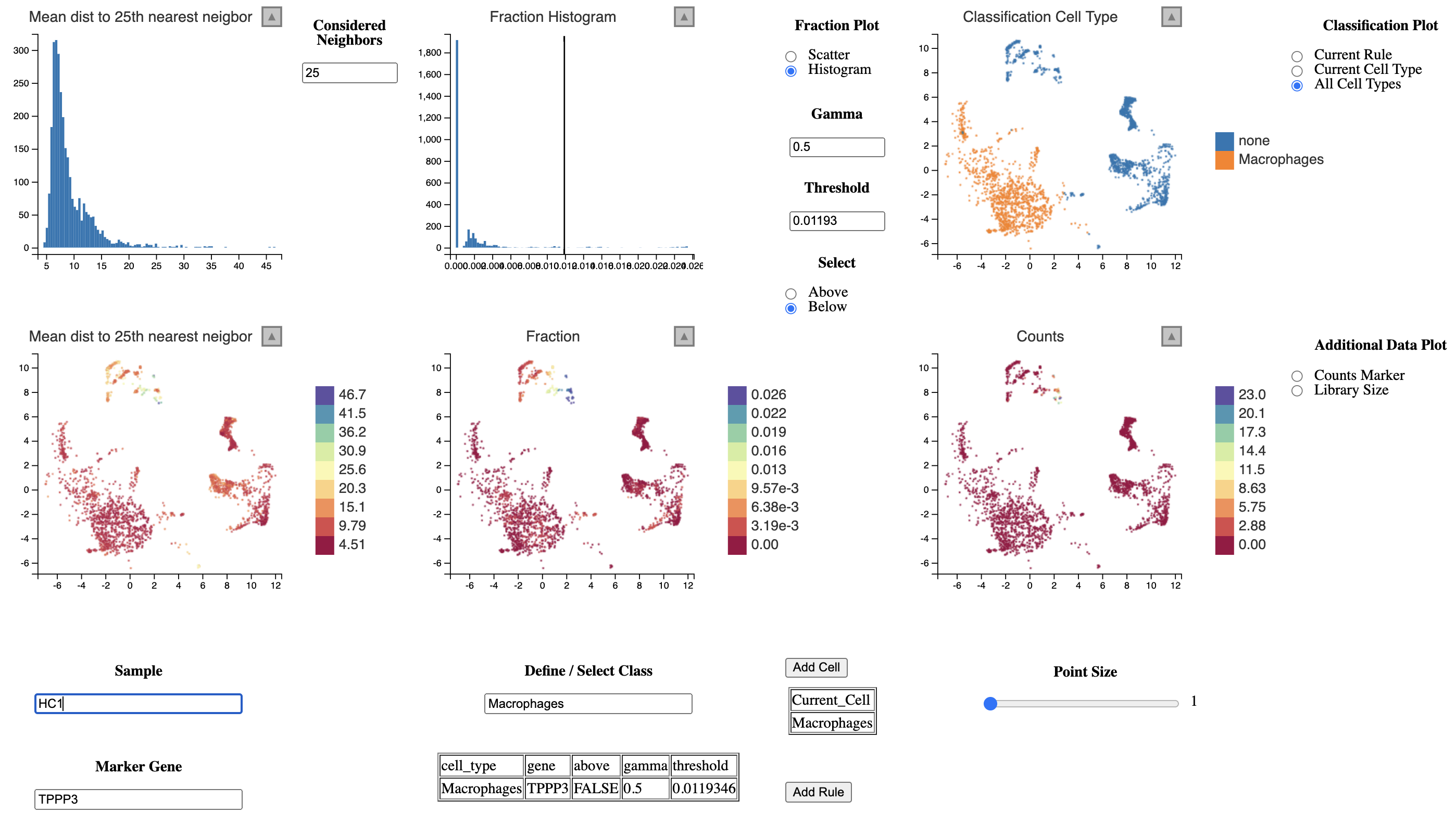
)The classification of macrophages in each sample could look like this. We define macrophages as cells which express CD68 and do not express CD3E (T-cells) or TPPP3 (Epithelial cells).
To go back and refine the annotation one should save the annotation and the rule list.
save(annotations, rules, file = "macrophage_annotation.RData")If one wishes to refine the annotation at some point, one can simply reload the application as done above and overwrite the annotations and rules objects by loading the .RData file.
load("macrophage_annotation.RData")Once we have annotated our cell type of interest we could perform for example differential gene expression analysis between the cells from the same cell type under different conditions (e. g. mild vs. severe COVID-19 infection). As we have only annotated macrophages so far, we will compare their expression profiles.
First, we will need to create pseudobulks for macrophages in each sample from the “M” (mild) and “S” (severe) samples.
# We want to compare macrophages in mild vs. severe COVID-19
mild_samples <- unique(cells$sample)[grepl("M", unique(cells$sample))]
head(mild_samples)
#> [1] "M1" "M2" "M3"
severe_samples <- unique(cells$sample)[grepl("S", unique(cells$sample))]
head(severe_samples)
#> [1] "S1" "S0" "S2" "S3" "S4" "S5"

cell_type = "Macrophages"

mild_matrix <- NULL
for (sample in mild_samples) {
  cell_type_barcodes <- annotations[[sample]][[cell_type]]$barcode
  mild_matrix <- cbind(mild_matrix, Matrix::rowSums(counts[, cell_type_barcodes]))
}
colnames(mild_matrix) <- mild_samples
head(mild_matrix)
#>              M1   M2 M3
#> AL627309.1    9    8  0
#> AL669831.5  163  133  1
#> FAM87B        9    4  0
#> LINC00115   120  199 14
#> FAM41C       54   64  1
#> NOC2L      1430 1292 53

severe_matrix <- NULL
for (sample in severe_samples) {
  cell_type_barcodes <- annotations[[sample]][[cell_type]]$barcode
  severe_matrix <- cbind(severe_matrix, Matrix::rowSums(counts[, cell_type_barcodes]))
}
colnames(severe_matrix) <- severe_samples
head(severe_matrix)
#>              S1  S0  S2  S3  S4  S5
#> AL627309.1   30  10   4   6   6   3
#> AL669831.5  174 114  40  32  61  70
#> FAM87B       11   0   0   0   0   0
#> LINC00115   375 132  29  59  37  65
#> FAM41C       86  82  22  50  37  44
#> NOC2L      2357 787 147 563 296 772
As we will be using DESeq2 for our differential gene epxression analysis, we have to create a small dataframe describing the samples (“coldata”).
coldata <- data.frame(sample=c(mild_samples, severe_samples))
coldata$condition <- ifelse(startsWith(coldata$sample, "M"), "mild", "severe")
coldata
#>   sample condition
#> 1     M1      mild
#> 2     M2      mild
#> 3     M3      mild
#> 4     S1    severe
#> 5     S0    severe
#> 6     S2    severe
#> 7     S3    severe
#> 8     S4    severe
#> 9     S5    severe
Now we can simply run DESeqDataSetFromMatrix.
suppressPackageStartupMessages(library(DESeq2))
dds <- DESeqDataSetFromMatrix(countData = cbind(mild_matrix, severe_matrix),
                                colData = coldata,
                                design = ~ condition)
#> converting counts to integer mode
#> Warning in DESeqDataSet(se, design = design, ignoreRank): some variables in
#> design formula are characters, converting to factors

dds <- DESeq(dds)
#> estimating size factors
#> estimating dispersions
#> gene-wise dispersion estimates
#> mean-dispersion relationship
#> final dispersion estimates
#> fitting model and testing
res <- results(dds)
And we could for example look at the genes assocatiated with the lowest adjusted p-values.
suppressPackageStartupMessages(library(dplyr))
res %>%
  as.data.frame %>%
  filter(padj < 0.1) %>%
  arrange(desc(log2FoldChange)) %>%
  select(-pvalue) %>%
  slice_head(n=10)
#>             baseMean log2FoldChange    lfcSE     stat         padj
#> IGKV3-11   4567.8948       28.74300 3.434250 8.369512 4.657479e-14
#> IGHV5-10-1 2336.6273       27.93190 3.434259 8.133311 2.832888e-13
#> IGKV1-9    1319.6604       27.13907 3.063320 8.859365 8.042479e-16
#> IGLV3-27   1222.8432       27.13060 3.434277 7.899948 1.394296e-12
#> IGHV1-46   1329.1049       26.95968 3.434274 7.850184 1.972134e-12
#> IGLV4-69   1046.2495       26.91493 3.434283 7.837134 2.084026e-12
#> IGHV3-74    973.1023       26.81567 3.434286 7.808223 2.541783e-12
#> IGLV2-23    814.9891       26.56442 3.434295 7.735043 4.005831e-12
#> IGKV1-6     777.4242       26.40558 3.434297 7.688786 5.641161e-12
#> IGHV1-24    655.1797       26.26125 3.434308 7.646738 7.385729e-12