R/LinkedCharts Tutorial:
Getting input from the web page
Load the data
Here, we introduced lc_input function and showed how to add radio buttons to the web page and then link them to a chart.
In this tutorial we are going to explore further possibilities of this function and show how you can make your app even more interactive.
As an example, we are going to create an app that allows one interectively change parameters of a UMAP
dimensionality reduction and see how they influence the embedding. The result will look like this
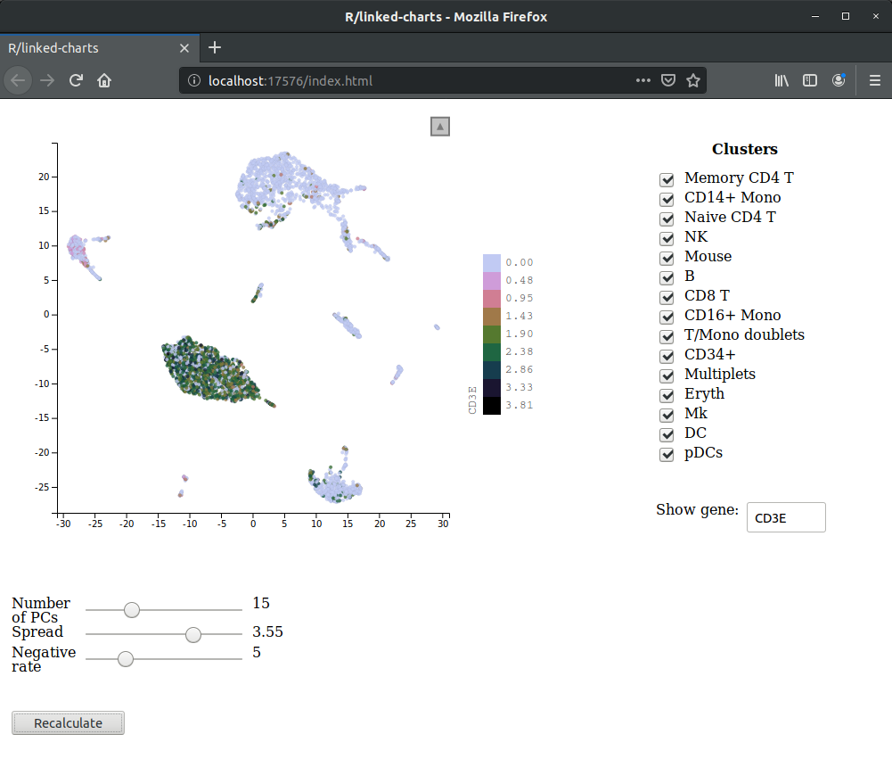
Unfortunately, for technical reasons, here, we can only show a screenshot, rather than righting the entire app in JavaScript like in all
previous tutorials. Yet, you can always download the full R code of the app an run it locally. Here, we are using the
same CiteSeq cord blood single-cell dataset by Stoecklin et al. (Nature Methods, 2017) as in other
tutorials, but these time we’ve used one of the Seurat’s tutorials to
preprocess the data. You can yourself follow couple of first steps from this tutorial (until cluster assignment), download
this script that has all the required preparations or directly load the Seurat object in
the .rds format.
We start with loading this object in the memory.
library(readr)

cbmc <- read_rds("seuratObject.rds")
cbmc
## An object of class Seurat
## 20501 features across 8617 samples within 1 assay
## Active assay: RNA (20501 features, 2000 variable features)
##  1 dimensional reduction calculated: pca
For this example, we are going to use only some of the information stored in this object, namely the PCA embedding, cluster assignment and normalized count matrix. So, for the sake of simplicity, we save these as separate variables and remove the Seurat object.
clusters <- cbmc@active.ident
pca <- cbmc@reductions$pca@cell.embeddings
X <- cbmc@assays$RNA@data

rm(cbmc)

head(clusters)
## CTGTTTACACCGCTAG CTCTACGGTGTGGCTC AGCAGCCAGGCTCATT GAATAAGAGATCCCAT GTGCATAGTCATGCAT TACACGACACATCCGG
##            Mouse            Mouse            Mouse            Mouse            Mouse            Mouse
## Levels: Memory CD4 T CD14+ Mono Naive CD4 T NK Mouse B CD8 T CD16+ Mono T/Mono doublets CD34+ Multiplets Eryth Mk DC pDCs
pca[1:5, 1:5]
##                       PC_1      PC_2      PC_3        PC_4       PC_5
## CTGTTTACACCGCTAG -35.40905 -3.420900 0.6320372  0.40590701  0.2410551
## CTCTACGGTGTGGCTC -34.99613 -3.912628 2.2778558 -0.10634510 -0.7120762
## AGCAGCCAGGCTCATT -35.86630 -3.944900 1.6303179  0.54025670  0.5464716
## GAATAAGAGATCCCAT -35.27736 -3.929127 1.1551277  0.48948888  0.5804452
## GTGCATAGTCATGCAT -34.19374 -3.277635 1.6822643  0.04960485  0.8715711
X[2000:2004, 1:5] #we are showing not the first rows to get some non-zero expression
## 5 x 5 sparse Matrix of class "dgCMatrix"
##         CTGTTTACACCGCTAG CTCTACGGTGTGGCTC AGCAGCCAGGCTCATT GAATAAGAGATCCCAT GTGCATAGTCATGCAT
## BCL11B                 .        0.3862658                .                .                .
## BCL2                   .        0.6642082                .                .                .
## BCL2A1                 .        .                        .                .                .
## BCL2L1                 .        .                        .                .                .
## BCL2L11                .        .                        .                .                .
Even though UMAP is a relatively fast dimensionality reductin tool, it still takes some time to recalculate an embedding for the full dataset. Since the goal of this example is to demonstrate LinkedCharts functionality and let users have fun while playing with all kinds of buttons, we are going to subsample the dataset.
cells <- sample(length(clusters), 2000)

clusters <- clusters[cells]
pca <- pca[cells, ]
X <- X[, cells]
Now, finally, let’s calculate a UMAP embedding using the first 15 principal components.
library(uwot)
npca <- 15

um <- umap(pca[, 1:npca])
head(um)
##                        [,1]      [,2]
## CTGCTGTAGTGTCCCG  -2.171477 -8.283055
## TCATTTGTCAGAGCTT -16.644293 -0.155554
## CACTCCAGTCTAAACC   0.906120 10.273386
## TGGGAAGGTTGCGCAC  -2.650380 -7.168352
## GGGTTGCAGGCAGTCA   2.304979  9.892189
## GCCAAATCAGTTCCCT  -2.498022 -7.678300
After that we are ready to make the central plot for our app.
library(rlc)

openPage(useViewer = FALSE, layout = "table1x2")

lc_scatter(x = um[1, ], y = um[2, ],
           size = 2, place = "A1")
## Chart 'A1' added.
## Layer 'Layer1' is added to chart 'A1'.
This gives you a boring all-black plot, not much different from one you can get with base plot() function. Step by step, we are going to add
various features to this basic plot to make it more informative and customizable.
Checkboxes
First, we add a way to select only some of the clusters. Later, this will allow us to recalculate the embedding with only selected cluster, but for now we just make not-selected cells transparent. To this end, let us add a set of checkboxes, each corresponding to a certain cluster.
useClusters <- levels(clusters)
useClusters
##  [1] "Memory CD4 T"    "CD14+ Mono"      "Naive CD4 T"     "NK"              "Mouse"           "B"               "CD8 T"           "CD16+ Mono"
##  [9] "T/Mono doublets" "CD34+"           "Multiplets"      "Eryth"           "Mk"              "DC"              "pDCs"
lc_input(type = "checkbox",
         labels = levels(clusters),
         value = TRUE,
         title = "Clusters",
         on_click = function(value) {
           useClusters <<- levels(clusters)[value]
           updateCharts("A1")
         },
         place = "A2")
## Chart 'A2' added.
useClusters is a variable to keep a list of currently selected clusters. We start with all clusters selected. Now lc_input with type = "checkbox"
comes in. It adds a set of checkboxes next to the main plot. labels is a vector of characters that are put next to each of the checkboxes. This
property also defines, how many checkboxes you want to get (by default, lc_input will create only one element). So, if you want, let say, 10
checkboxes with no labels, you need to pass a vector of 10 empty strings to this property labels = rep("", 10). We also put a title above our
checkboxes with title = "Clusters".
value is very important property for ane lc_input object, since it describes the current state of the input block. It behaves differently for
different types of inputs. For instance, state of checkboxes is described by vector of logicals: TRUE for a checked box and FALSE for an not checked
one. lc_input of type radio is described by a single number - an index of the selected button. State of range and text is a vector of current values of each element. In case of range it is always a vector of numerics, while text uses a character vector with possible NA, if the
correspoding text field is empty. Finally, lc_input with type = "button" doesn’t have a state as such, but a callback function receives
a label (not index!) of the clicked button.
This all may sound complicated at first, but try to play with this simple expample to get a feeling of it. It will print current state of
lc_input, whenever you enter text, click button, select checkbox or radio button.
lc_input(type = "checkbox", labels = paste0("el", 1:5), on_click = function(value) print(value),
         value = T)
lc_input(type = "radio", labels = paste0("el", 1:5), on_click = function(value) print(value),
         value = 1)
lc_input(type = "text", labels = paste0("el", 1:5), on_click = function(value) print(value),
         value = c("a", "b", "c", "e", "d"))
lc_input(type = "range", labels = paste0("el", 1:5), on_click = function(value) print(value),
         value = 10, max = c(10, 20, 30, 40, 50), step = c(0.5, 0.1, 1, 5, 25))
lc_input(type = "button", labels = paste0("el", 1:5), on_click = function(value) print(value))
value of the input block can be used in two directions. It is what a callback (on_click or on_change) function gets, when user interacts
with the input elements. And it is also what you can pass to the input block from the R session to change its current state. For examle, here with
value = TRUE (equivalent to value = rep(TRUE, length(levels(clusters)))) we make sure that in the beginning all the checkboxes are checked.
The callback on_click function is called each time user checks or unchecks a checkbox. As it was mentioned above, it gets a verctor of TRUE and
FALSE, which we use to update a list of currently selected clusters and then update the main plot. For lc_input on_click and on_change are
complete synonims. You can use whichever one of them you find more intuitive.
Now, it’s only left to make use of our useClusters variable. So we replace our main plot with
lc_scatter(dat(opacity = ifelse(clusters %in% useClusters, 0.8, 0.1)),
           x = um[, 1], y = um[, 2],
           size = 2, place = "A1")
## Layer 'Layer1' is added to chart 'A1'.
We have added another property opacity which makes cells from not selected clusters more transparent than others.
You may have noticed, that the previous version of the main plot didn’t have the dat function, but here it appears.
The trick is that parameters inside the dat function are recalculated on every update call, while those outside are
evaluated only once. If you have any doubts, you can always put everything iside the dat function.
Text fields
lc_input of type text adds one or several text fields to the web page. Here, we will make one that allows user to enter a gene name
and immediately see its expression on the plot.
selGene <- "CD3E"

lc_input(type = "text",
         label = "Show gene: ",
         place = "A2",
         chartId = "geneBox",
         value = selGene,
         on_change = function(value) {
           if(value %in% rownames(X)) {
             selGene <<- value
             updateCharts("A1", updateOnly = "ElementStyle")
           }
         }
)
## Chart 'geneBox' added.
This code adds one text field labeled Show gene:, with initial value CD3E (stored in selGene). Whenever users enters a new gene name, it checks
whether it is really a name of a gene, which expression is stored in the count matrix, and, if so, resets the selGene variable and updates the main
plot. updateOnly here is an optional parameter that tells LinkedCharts to change only styling of points, but not there position of number. In some
cases, it may safe performance time.
Not so obvious thing here, is why we defined chartId of the lc_input block. As you can see, we put in the same table cell A2 as the set of checkboxes.
By default, LinkedCharts set an ID of each chart the same as ID of its container (A2 in this case). But since we already have a chart with ID A2,
this will cause replacing our checkboxes with a text field. To avoid that we explicitly specify another ID. Now, text field is added under the
checkboxes.
Now it’s time for another change in the main plot
lc_scatter(dat(opacity = ifelse(clusters %in% useClusters, 0.8, 0.1),
               colourLegendTitle = selGene,
               colourValue = X[selGene, ],
               x = um[, 1], y = um[, 2]),
           size = 2,
           palette = rje::cubeHelix(n = 11)[9:1],
           place = "A1")
## Layer 'Layer1' is added to chart 'A1'.
Here, we used normalized expression as colourValue and gene name as legend’s title (colourLegendTitle). We also change default palette to Cube Helix
just to make it look nicer.
If user enters a gene that doesn’t exist, nothing happens. However it may be nice to tell user why there are no changes in the main plot.
lc_html can help us here. This fucntion simply places a piece of HTML code to the web page.
display <- "none"
lc_html(dat(content = paste0("<p style='color: red; display: ", display, "'>There is no such gene</p>")),
        place = "A2", chartId = "warning")
## Chart 'warning' added.
This code adds a paragraph with text “There is no such gene” once again to the A2 table cell. For this paragraph we set two style attributes.
color: red makes the text red and display: none makes the parahraph hidden. As you can notice, we assume that this attribute may
change in time and store it in a separate variable. Now we need to make changes in the text field callback function.
lc_input(type = "text",
         label = "Show gene: ",
         place = "A2",
         chartId = "geneBox",
         value = selGene,
         on_change = function(value) {
           if(value %in% rownames(X)) {
             display <<- "none"
             selGene <<- value
             updateCharts("A1", updateOnly = "ElementStyle")
           } else {
             display <<- "undefined"
           }
           updateCharts("warning")
         }
)
## Chart 'geneBox' added.
display here equals none if gene with user specified name exists and undefined otherwise. In any case, lc_html gets updated with the new
display value.
Ranges and buttons
Next type of lc_input is range. It is a slider that is used to roughly specify a numeric value. Besides abovementioned parameters, ranges have three
more. min and max set minimal and maximal values that can be selected with a slider (defaults are 0 and 100 respectively). step is a stepping
interval between allowed values that can be set by the slider.
In this example we will play with just three parameters of the embedding. The first one is number of principal components that is used to for
dimensionality reduction. Our default value 15 was set above (stored in npca). We want this parameter to be integer and allow it to accept values
from 2 to 50. spread determines how clustered/clumped the embedded points are. Defualt value is 1. Let it be somewhere between 0.01 and 5 with step
0.01. Negative rate (negRate) in some sense defines how strongly embedded points are repelled from each other. It is going to vary from 0.5 to 20
with default value 5.
Let’s sum it all up in some R code
negRate <- 5
spread <- 1

lc_input(type = "range",
         label = c("Number of PCs", "Spread", "Negative rate"),
         width = 300,
         value = c(15, 1, 5),
         min = c(2, 0.01, 0.5),
         max = c(50, 5, 20),
         step = c(1, 0.01, 0.5),
         on_change = function(value) {
           npca <<- value[1]
           spread <<- value[2]
           negRate <<- value[3]
         })
## Chart 'Chart5' added.
We don’t use place parameter, which means that this block of ranges will be put just under all the existing plots. There are also no changes
made to the main plot in the callback function. Recalculating of the embedding takes some time and therefore we want to do it only after user
specifies all the parameters. So we add a button that one need to click to trigger recalculation.
lc_input(type = "button",
         label = "Recalculate",
         on_click = function(value) {
           print("Recalculation started. Please, wait...")
           inclCells <<- clusters %in% useClusters
           um <<- umap(pca[inclCells, 1:npca], negative_sample_rate = negRate, spread = spread)
           print("Recalculation finished")
           updateCharts("A1")
         })
## Chart 'Chart6' added.
Let’s go line by line through the callback function.
First, since recalculating will take some time, we want user to be aware of this and print a message that the system is currently busy. This message will appear in the R console. Another way is to do it directly on the web page, but we are going to leave it as an exercise for the reader. Next, we check which cells belong to the selected clusters. Then we calculate a new embedding using only those cells and all the parameters set by the sliders. Now we can tell user that calculations are finished and update the main plot.
And finally, there is just one more thing left. We need to make sure, that only the cells from selected cluters are now displayed on the plot. We
also will need and initial value for inclCells (TRUE for all the cells).
inclCells <- rep(T, ncol(X))

lc_scatter(dat(opacity = ifelse(clusters[inclCells] %in% useClusters, 0.8, 0.1),
               colourLegendTitle = selGene,
               colourValue = X[selGene, inclCells],
               x = um[, 1], y = um[, 2]),
           size = 2,
           palette = rje::cubeHelix(n = 11)[9:1],
           place = "A1")
## Layer 'Layer1' is added to chart 'A1'.
Here, we are subsetting our cells for defining opacity and colourValue.
By now, if you’ve followed all the steps of this tutorial you should have a fully functional app in your browser. You can also download the full R code.