R/LinkedCharts Tutorial:
A multi-coloured t-SNE plot
In this example, we continue our exploration of the CiteSeq cord blood single-cell dataset by Stoecklin et al. (Nature Methods, 2017). If you haven’t read the first part yet, please go there first.
This is what we are aiming for:
In this app, you can assign a colour channel to each antibody, and so explore the identities of the cells in a colourful manner. If you want to try this out first before reading the details, here is the complete code. It’s less than a page of R.
Loading the data
The CiteSeq method presented by Stoecklin et al. in their paper is a way to simultaneously sequence the transcriptome and the “epitome” of thousands of single cells, where “epitome” means a collection of surface markers (epitopes) of the cells: they conjugated antibodies for 13 different blood cell surface markers with DNA oligomers, which they sequenced alongside the cell’s own transcripts, thus getting counts of sequencing reads from the labelled antibody molecules, which they denote “antibody-derived tags” (ADTs).
We have already explored the transcriptome data in the first part of this tutorial. Now, we will use the epitome data to learn more about the cells’ identities.
We start by loading again the rlc library and the CiteSeq data file that we have prepared in the first part, and which you can download here.
library( rlc )

load( "citeseq_data.rda" )
We also download the epitome data table (ADT table) from GEO.
download.file( "ftp://ftp.ncbi.nlm.nih.gov/geo/series/GSE100nnn/GSE100866/suppl/GSE100866_CBMC_8K_13AB_10X-ADT_umi.csv.gz",
   "GSE100866_CBMC_8K_13AB_10X-ADT_umi.csv.gz" )

countMatrixADT <- as.matrix( read.csv( gzfile( "GSE100866_CBMC_8K_13AB_10X-ADT_umi.csv.gz" ), row.names=1 ) )
We first subset the matrix to only those rows that describe the cells that we had retained when filtering the RNA count matrix:
countMatrixADT <- countMatrixADT[ , colnames(countMatrix) ]
We now have UMI count values for antibody-derived tags (ADTs) from antibodies against 13 epitopes, for ~8000 cells. Here are the first 4 cells:
countMatrixADT[ , 1:4 ]
##        TACAGTGTCTCGGACG GTTTCTACATCATCCC ATCATGGAGTAGGCCA GTACGTATCCCATTTA
## CD3                  36               34              370               49
## CD4                  28               21             1706               38
## CD8                  34               41             9559               52
## CD45RA              228              228           102390              300
## CD56                 26               18             1518               48
## CD16                 44               38             4617               51
## CD10                 41               48              363               48
## CD11c                25               16             8204               41
## CD14                 44               57             4402               89
## CD19                 24               27              988               29
## CD34                 24              230              422               57
## CCR5                 28               24              879               42
## CCR7                 24               27              239               36
A multi-channel flourescent t-SNE plot
Last time, we calculated from the RNA-Seq data a t-SNE plot. If we want to know which of these cells are T cells, we cold colour the cells by the strength of expression of the T-cell marker CD3:
unitrange <- function( x )
  ( x - min(x) ) / ( max(x) - min(x) )

plot( tsne$Y,
   col = rgb( unitrange( log( countMatrixADT[ "CD3", ] ) ), 0, 0 ),
   asp = 1, pch=20, cex=.5 )
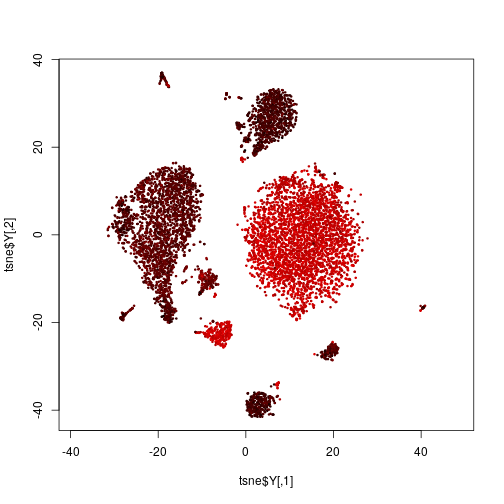
Here, we have defined a function unitrange, which simply takes a vector of numbers (here, the logarithmized expression of the CD3 epitope) and scales them such that the smallest number becomes 0 and the largest 1. This is what the rgb function wants: three numbers, all between 0 and 1, which is uses to mix a colour with the specified amount of red (R), green (G) and blue (B). (If you are unfamiliar with the RGB color model, look it up, e.g., on Wikipedia.)
To see, for example, both T cells and B cells on one glance, we could continue to use the red channel for CD3 and the green channel for CD19, a B-cell marker:
plot( tsne$Y,
   col = rgb(
     unitrange( log( countMatrixADT[ "CD3", ] ) ),    # red channel:   T cell marker
     unitrange( log( countMatrixADT[ "CD19", ] ) ),   # green channel: B cell marker
     0 ),                                             # blue channel:  not used
   asp = 1, pch=20, cex=.5 )
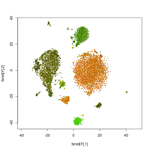
Is the big cluster on top, with the brownish red-green mix now a B or a T cell, or something else. It would be nice to be able to quickly explore all the markers by attaching to them red, green or blue “virtual flourophores” on the click of a button. This is what the app on the top of the page allows us to do.
Interactive input
Those, who already have had a look at one of the previous tutorials, may guess, how to make such a scatter plot in
linked-charts with lc_scatter function. Here, we’ll just show the result.
red   <- "off"
green <- "off"
blue  <- "off"

lc_scatter(
   dat(
      x = tsne$Y[,1],
      y = tsne$Y[,2],
      colour = rgb(
          if( red == "off" )   0 else unitrange(log( countMatrixADT[red, ] )),
          if( green == "off" ) 0 else unitrange(log( countMatrixADT[green, ] )),
          if( blue == "off" )  0 else unitrange(log( countMatrixADT[blue, ] )) ),
      size = 1 ))
## Chart 'Chart5' added.
## Layer 'Layer1' is added to chart 'Chart5'.
We created three variables red, green and blue to store the markers for each colour channel. Initially they all are off and all the points on
the scatter plot are black. Now, one can manually change them and run updateCharts() like this.
red <- "CD3"
green <- "CD19"
updateCharts()
Yet, what would be really great to do the same in an interactive manner, simply by clicking. This can be done with the help of lc_input function
that allows to add HTML [input](https://www.w3schools.com/tags/tag_input.asp) tags on the page and handle their responses. linked-charts supports
five types of input: "text", "radio", "range", "checkbox" and "button". For this example we would need three sets of radio buttons - one for each
colour channel. Let’s put it side by side next to the scatter plot.
openPage(FALSE, layout = "table1x4")

red   <- "off"
green <- "off"
blue  <- "off"

lc_scatter(
  dat(
    x = tsne$Y[,1],
    y = tsne$Y[,2],
    colour = rgb(
      if( red=="off" )   0 else unitrange(log( countMatrixADT[red,] )),
      if( green=="off" ) 0 else unitrange(log( countMatrixADT[green,] )),
      if( blue=="off" )  0 else unitrange(log( countMatrixADT[blue,] )) ),
    size = 1 ),
  place = "A1" )
## Chart 'A1' added.
## Layer 'Layer1' is added to chart 'A1'.
buttonRows <- c("off", rownames(countMatrixADT))

lc_input(type = "radio",
         labels = buttonRows,
         title = "Red",
         value = 1,
         width = 100,
         on_click = function(value) {
            red <<- buttonRows[value]
            updateCharts("A1")
         },
         place = "A2")
## Chart 'A2' added.
lc_input(type = "radio",
         labels = buttonRows,
         title = "Green",
         value = 1,
         width = 100,
         on_click = function(value) {
            green <<- buttonRows[value]
            updateCharts("A1")
         },
         place = "A3")
## Chart 'A3' added.
lc_input(type = "radio",
         labels = buttonRows,
         title = "Blue",
         value = 1,
         width = 100,
         on_click = function(value) {
            blue <<- buttonRows[value]
            updateCharts("A1")
         },
         place = "A4")
## Chart 'A4' added.
Here, we create 1x4 table and put our scatter plot in the leftmost cell. Three other cells are occupied by the sets of radio buttons. For each of them
we set a required property type, which must be one of c("text", "radio", "range", "checkbox", "button"), to "radio". Then we need to specify an
array of labels to be printed next to our radio buttons. In this example, we use all available markers and off value, which is stored in the
buttonRows variable.
buttonRows
##  [1] "off"    "CD3"    "CD4"    "CD8"    "CD45RA" "CD56"   "CD16"
##  [8] "CD10"   "CD11c"  "CD14"   "CD19"   "CD34"   "CCR5"   "CCR7"
lc_input uses labels to define the number of required elements, which is 1 by default. So even if you don’t want to any text next to your
radiobuttons or checkboxes, you are still requeired to pass an array of empty strings to this property.
value sets current value for an input element. For a set of radio buttons, it’s a number of the checked button. Here, we use this property to set the
initial value, but in other applications you can also use this property to control the state of your inputs from the R session.
The on_click property works the same way as it does in all other charts in the rlc library. Whenever user clicks on one of the buttons, this function
is called. As an arguments it gets current value of the input block (for radio buttons it’s a number of the checked button). So we assign
corresponding value to
the variable of the corresponding colour channel and update the A1 chart (the scatter plot). If you know how to use HTML input tags, you may know
that generally they use the onchange attribute instead of onclick, which means that the event is fired not when user clicks on the element, but
only when its value is changed. Internally rlc does the same, however to make it less confusing, we decided to keep the same property name. You can
also use on_change instead of on_click if you find this more intuitive. For lc_input the two are complete synonims.
Finally, we give a title to each button set and change its width to 100 pixels to make them less spread (the default width is 200 pixels).